Field data inversion (“Koenigsee”)

This minimalistic example shows how to use the Refraction Manager to invert a field data set. Here, we consider the Koenigsee data set, which represents classical refraction seismics data set with slightly heterogeneous overburden and some high-velocity bedrock. The data file can be found in the pyGIMLi example data repository.

# We import pyGIMLi and the traveltime module.

import matplotlib.pyplot as plt
import pygimli as pg
import pygimli.physics.traveltime as tt

The helper function pg.getExampleData downloads the data set to a temporary location and loads it. Printing the data reveals that there are 714 data points using 63 sensors (shots and geophones) with the data columns s (shot), g (geophone), and t (traveltime). By default, there is also a validity flag.

data = pg.getExampleData("traveltime/koenigsee.sgt", verbose=True)
print(data)

Data: Sensors: 63 data: 714, nonzero entries: ['g', 's', 't', 'valid']

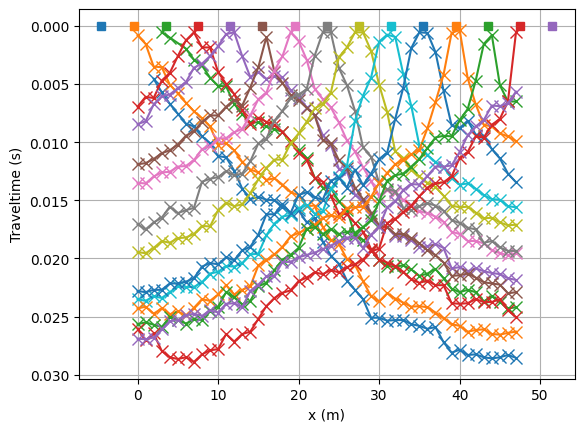
Let’s have a look at the data in the form of traveltime curves.

fig, ax = plt.subplots()
lines = tt.drawFirstPicks(ax, data)

We initialize the refraction manager.

mgr = tt.TravelTimeManager(data)

# Alternatively, one can plot a matrix plot of apparent velocities which is the
# more general function also making sense for crosshole data.

ax, cbar = mgr.showData()

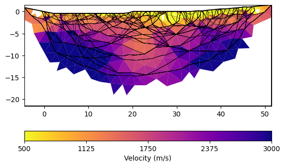
Finally, we call the invert method and plot the result.The mesh is created based on the sensor positions on-the-fly.

mgr.invert(secNodes=3, paraMaxCellSize=5.0,
           zWeight=0.2, vTop=500, vBottom=5000, verbose=1)

fop: <pygimli.physics.traveltime.modelling.TravelTimeDijkstraModelling object at 0x2929a7290>
Data transformation: <pygimli.core._pygimli_.RTrans object at 0x2916dbab0>
Model transformation (cumulative):
         0 <pygimli.core._pygimli_.RTransLogLU object at 0x297918200>
min/max (data): 3.5e-04/0.03
min/max (error): 3%/3%
min/max (start model): 2.0e-04/0.002
--------------------------------------------------------------------------------
inv.iter 0 ... chi² =  156.33
--------------------------------------------------------------------------------
inv.iter 1 ... chi² =   12.31 (dPhi = 91.50%) lam: 20.0
--------------------------------------------------------------------------------
inv.iter 2 ... chi² =    8.91 (dPhi = 27.37%) lam: 20.0
--------------------------------------------------------------------------------
inv.iter 3 ... chi² =    6.65 (dPhi = 24.90%) lam: 20.0
--------------------------------------------------------------------------------
inv.iter 4 ... chi² =    5.97 (dPhi = 9.74%) lam: 20.0
--------------------------------------------------------------------------------
inv.iter 5 ... chi² =    5.77 (dPhi = 3.11%) lam: 20.0
--------------------------------------------------------------------------------
inv.iter 6 ... chi² =    5.61 (dPhi = 2.58%) lam: 20.0
--------------------------------------------------------------------------------
inv.iter 7 ... chi² =    4.68 (dPhi = 15.30%) lam: 20.0
--------------------------------------------------------------------------------
inv.iter 8 ... chi² =    4.24 (dPhi = 8.78%) lam: 20.0
--------------------------------------------------------------------------------
inv.iter 9 ... chi² =    3.97 (dPhi = 5.67%) lam: 20.0
--------------------------------------------------------------------------------
inv.iter 10 ... chi² =    3.79 (dPhi = 4.16%) lam: 20.0
--------------------------------------------------------------------------------
inv.iter 11 ... chi² =    3.71 (dPhi = 1.87%) lam: 20.0
################################################################################
#                Abort criterion reached: dPhi = 1.87 (< 2.0%)                 #
################################################################################

1090 [860.2734766657787,...,2649.3970266259444]

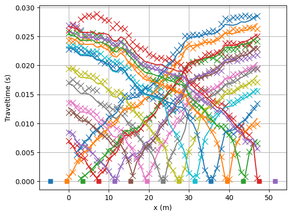
Look at the fit between measured (crosses) and modelled (lines) traveltimes.

mgr.showFit(firstPicks=True)

You can plot only the model and customize with a bunch of keywords

ax, cbar = mgr.showResult(logScale=False, cMin=500, cMax=3000, cMap="plasma_r",
                          coverage=mgr.standardizedCoverage())
rays = mgr.drawRayPaths(ax=ax, color="k", lw=0.3, alpha=0.5)

# mgr.coverage() yields the ray coverage in m and standardizedCoverage as 0/1

You can play around with the gradient starting model (vTop and vBottom arguments) and the regularization strength lam and customize the mesh.